
Asset And Liability Management
Interest Rate Risk
Interest Rate Risk
Interest Rate Risk is the risk to the bank's profitability caused by changing rates and the balance between assets and liabilities. Financial instruments on each side of the balance sheet have different terms related to pricing and tenure, and variations on both can have effects on bank revenues.
For example, in an environment where you have a fixed rate asset funded by a variable rate liability and the rates are rising, the bank's revenue will reduce. And if the asset contract does not allow any rate change, the bank will have to minimise this impact.
Net Interest Income (NII) impact due to Interest Rates
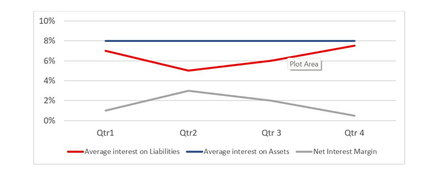
Normally, banks assets (loans to customers) have long maturity and more fixed interest rates, while the liabilities are short term and varies according to market conditions. The graph below shows how the net interest rate is affected when the interest rate on liabilities varies, considering a fixed interest rate on assets.
Interest Rate changes will affect the Balance Sheet through:
- Liquidity – changes in investment instruments
- Credit – increase in delinquency
- Foreign exchange – change in relative values
- Cost of doing business – price changes
Here is where the external factors analysis, mentioned earlier in the module, plays an important role in the effort to mitigate the interest rate risk, as interest rates may move up or down depending on the economy.
Basis Risk
Different financial instruments may be linked to various reference rates, potentially leading to what is known as basis risk. This occurs when these reference rates fluctuate in different directions or with varying degrees of change. For instance, a bank may have a mortgage portfolio where interest is calculated based on an interbank base rate, while the funding for this portfolio relies on financial instruments tied to a government bond rate. If these reference rates move in different directions, speed or degree of variation, it can impact the portfolio's profitability.
The below chart shows an example where two different references were used on the asset and liability side of the deal. The chart shows how LIBOR-based mortgage rates and government bond yields fluctuate over time. The basis risk spread (difference between LIBOR and the government bond yield) varies, highlighting the imperfect correlation between the two rates.
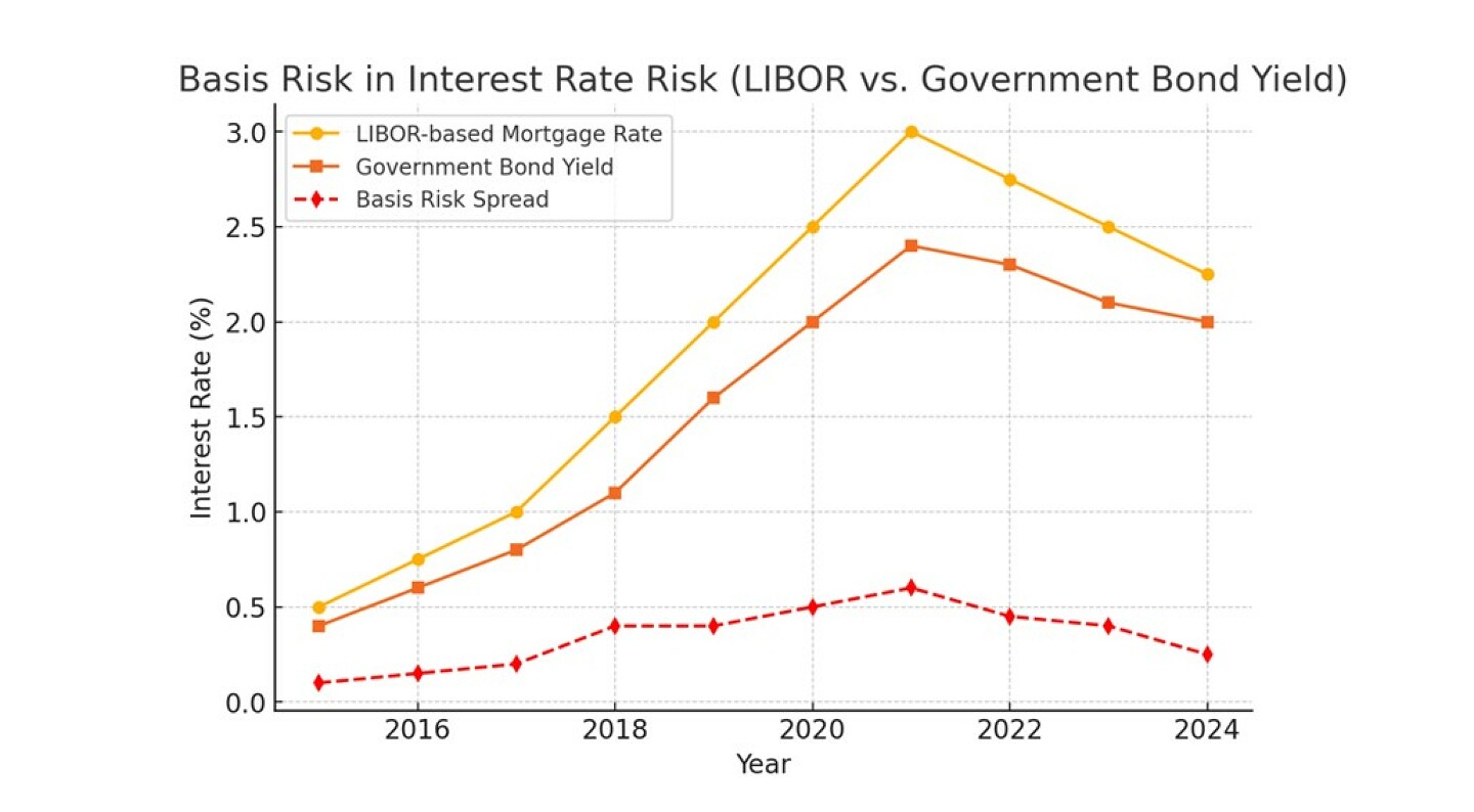
The bank's mortgages are tied to LIBOR but its funding is linked to government bond yields, and unexpected fluctuations in the spread can affect profitability. In the example, if LIBOR rises faster than the government bond yield, the bank benefits. But if LIBOR falls sharply while funding costs remain stable, the bank loses income on mortgages.
How to avoid or minimise such a situation?
Use interest rate swaps or basis swaps to hedge against misalignment. A swap is a derivative contract between two parties to exchange interest rate payments over a set period. It allows financial institutions, corporations, and investors to hedge interest rate risk or speculate on rate movements. It works when two parties agree to exchange cash flows based on different interest rate benchmarks. One faces the fixed rate and the other the variable one. In the swap only the difference is exchanged, positive or negative.
Another way to avoid the basis rate issue is by aligning loan pricing and funding sources with the same reference rate when possible. Actively monitor interest rate correlations and adjust risk management strategies accordingly.
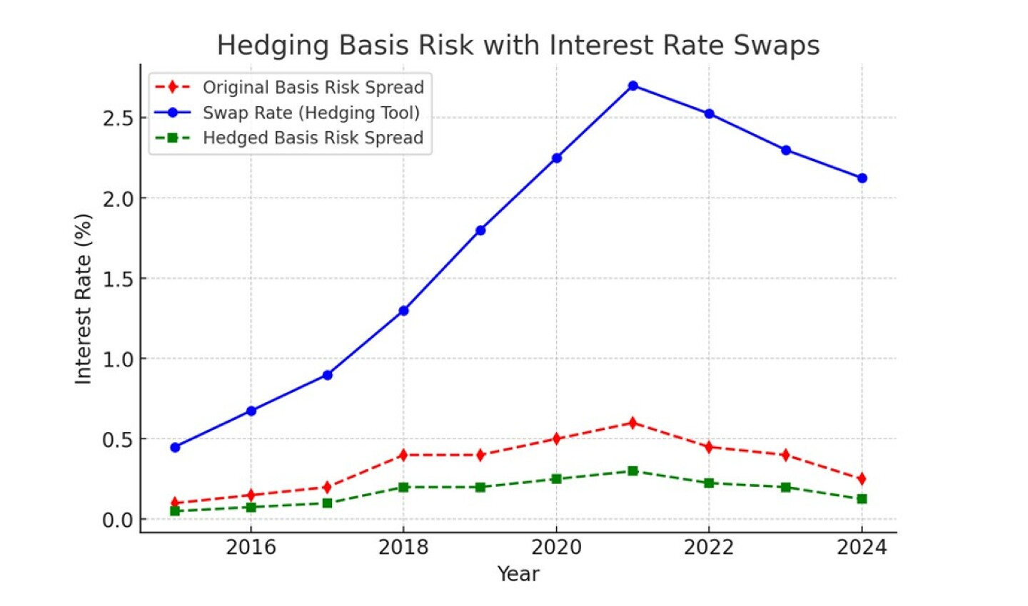
Another aspect that can create a mismatch is the fact that some instruments allow optionality, like pre-payments of loans. It is important when using fixed-rate funding mechanisms to fund loans, when possible, to avoid optionality, avoiding any future surprises caused by external factors.
We had recently an emblematic case of a bank that by lacking the proper ALM suffered a bank run. The collapse of Silicon Valley Bank (SVB) in March 2023, which we covered in Governance, was one of the most significant bank failures since the 2008 financial crisis. It was a classic bank run, where depositors panicked and rushed to withdraw their funds, leading to SVB's insolvency and regulatory takeover. SVB's failure was not due to fraud but rather poor risk management, rising interest rates, and a fast-moving bank run. The case highlights the importance of liquidity risk management, hedging, and depositor confidence in banking stability.
Assessing Interest Rate Risk
There are many ways to assess a bank's Interest Rate Risk.
Gap analysis – this is when the bank lists the various assets and funding liabilities by maturity and assesses any existing gap between the two. Such analysis is simple and provides a clear understanding of potential mismatches changes affecting the Net Interest Income (NII).
Gap Analysis Formula:
Gap = Rate-Sensitive Assets minus Rate-Sensitive Liabilities
Positive Gap (> 0): More rate-sensitive assets than liabilities -> Profits increase when rates rise.
Negative Gap (< 0): More rate-sensitive liabilities than assets->Profits decrease when rates rise.
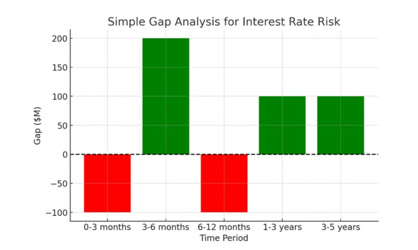
The table and chart provide a simple example of Gap Analysis for Interest Rate Risk.
The Negative Gap (Red Bars) is 0-3 Months & 6-12 Months
The bank has more rate-sensitive liabilities (RSL) than rate-sensitive assets (RSA).
This means that if interest rates increase, the bank's cost of funding rises more than its income, leading to a negative impact on net interest income.
The Positive Gap (Green Bars) is 3-6 Months & Long-Term Periods (1-5 Years)
Here, the bank has more rate-sensitive assets than liabilities. If interest rates rise, the bank benefits because its income from loans increases more than its cost of deposits. Like many index and analysis tools, Gap analysis has issues, such as ignoring rollovers, repricing within the band periods analysed, or any optionality risk.
PVBP is Present Value for One Basis Point fluctuation, an analysis of the portfolio and various instruments of what would be the effect of a 1bp variation. Of course, the higher the PVBP, the higher the risk, and the higher the exposure of the bank to an interest rate variation. A lower PVPB means less exposure on rate movements, helping the bank to define how much a bond or a loan portfolio will gain or lose with small rate fluctuations.
A negative figure shows the bank will lose money if rates rise, and a positive figure shows the bank will make money if the rate rises. PVBP can be used for assets and liabilities or specific portfolios, and the aggregate figure shows the effect on the bank NII.
The PVBP helps to calculate how much to pay to hedge a portfolio or a balance sheet.
Example of PVBP on a Loan Portfolio
Loan Portfolio Notional: $200 million
Modified Duration: 7 years
Basis Point Change: 0.01% (1 basis point, or 0.0001)
PVBP Calculation:
PVBP=$200m x 7 x 0.0001=$140,000 PVBP
So, if interest rates increase by 1 basis point (0.01%), the loan portfolio loses $140,000 in value. If it decreases by 1 basis point (0.01%), the loan portfolio gains $140,000 in value.
Again, as with any index to measure risks, there are weaknesses. Like GAP it cannot predict optionality, and is complex to calculate as it has to be calculated on different bands up to maturity. Focused on MTM, and difficult to apply on instruments without a maturity date, it can only apply to small interest variations.
Stress Testing – by creating different scenarios and applying their consequences to a portfolio or the Balance sheet, a bank can understand the effects of interest rate changes on the Net Interest Income (NII). A strength of Stress Testing is that optionality can be incorporated as well as different values for different rate parameter basis (basis risk). It is a complex method and will require a clear understanding of the main instruments in the portfolio or balance sheet, how each one behaves when interest rates change, and the impact on the reference rates. It is the only way to predict likely future outcomes.
VaR – value at risk estimates the potential loss within a certain percentage of confidence, resulting from movements in the market on rates or price, in a certain period.
VaR uses historical data behaviour of rates and prices to define the potential future losses. It is normally done over two years, which can produce 520 potential Profit and Loss (P&L) results, and define 99% confidence in the maximum loss that a portfolio or a Balance Sheet can face.
The bank lists the last two years' P&L results and the percentage of each result until the total gives 99%, which will define the maximum loss. It could be 95%, but this depends on the certainty based on the past that a manager wants to achieve. This is a backwards view to reflect the present.
There are a few different statistical methods to calculate the VaR and we will not dwell on them here. We are presenting a simple method based on the standard deviations that can be calculated in Microsoft Excel. To do it manually would be very time-intensive.
To use the Microsoft Excel method, you will need to provide all the rates for the defined period of time to calculate the standard deviation and apply the formula:
VaR = Portfolio Value x Duration x Interest Rate Volatility x Z
Where:
Portfolio Value = Total value of the portfolio analysed
Modified Duration = Sensitivity of the portfolio to interest rate changes
Interest Rate Volatility = Standard deviation of interest rate changes
Z = score based on the confidence level (e.g., 1.645 for 95% or 2.33 for 99%)
An Example of calculation of VaR for Interest Rate Risk
A bank has a $200 million loan portfolio with:
Modified Duration = 7 years
Interest Rate Volatility = 1.5% (calculate the standard deviation for the defined period)
Confidence Level = 95% (Z = 1.645)
Time Horizon = 1 day
VaR = $200 m x 7 x 0.015 x 1.645 x square root of 1/252 = $2,172,880 (we multiply by square root of 1/252 due to the one day duration)
VaR = $2.17m
What the number means: There is a 95% probability that the portfolio will not lose more than $2.17million in a single day due to interest rate movements. However, in extreme cases (5% probability), the loss could be higher. Banks can use derivatives (swaps, futures, or options) to mitigate risk based on VaR.
VaR = $2.17m
What the number means: There is a 95% probability that the portfolio will not lose more than $2.17m million in a single day due to interest rate movements. However, in extreme cases (5% probability), the loss could be higher. Banks can use derivatives (swaps, futures, or options) to mitigate risk based on VaR.
Again, as with any measuring instrument it has weaknesses. As mentioned earlier, it looks backwards, only providing the mean analysis over the period, and not a point-in-time worst potential loss. Depending on the new economic environment, the expected loss could get much worse.
EVE – Economic Value of Equity, required in Basel II, is basically to measure the impact of a plus or minus 200 bps variation in interest rates within the bank's balance sheet, and how it will affect the various instruments of the overall balance sheet. One way of doing this is through cash flow analysis by maturity and terms of instrument. EVE requires a complex system, similar to the stress testing modeling.
By now, you should understand that no one single measure predicts and calculates all the risks. A bank should pick and use a combination of them.